4 Simple Techniques For Excel Shortcuts

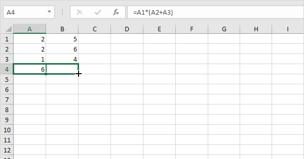
By pressing ctrl+shift+center, this will certainly calculate as well as return worth from multiple varieties, instead of simply individual cells contributed to or increased by each other. Determining the amount, product, or quotient of individual cells is easy-- simply make use of the =SUM formula as well as get in the cells, values, or variety of cells you wish to perform that arithmetic on.

If you're seeking to find overall sales revenue from a number of marketed devices, as an example, the variety formula in Excel is excellent for you. Here's exactly how you would certainly do it: To start using the variety formula, kind "=SUM," as well as in parentheses, get in the initial of two (or three, or 4) series of cells you would love to increase with each other.

This stands for multiplication. Following this asterisk, enter your 2nd series of cells. You'll be multiplying this second series of cells by the initial. Your progress in this formula should now appear like this: =SUM(C 2: C 5 * D 2:D 5) Ready to push Go into? Not so quick ... Because this formula is so complex, Excel gets a different key-board command for selections.

This will identify your formula as a range, covering your formula in support characters as well as efficiently returning your product of both arrays incorporated. In profits estimations, this can lower your effort and time considerably. See the final formula in the screenshot over. The MATTER formula in Excel is denoted =COUNT(Beginning Cell: End Cell).

As an example, if there are eight cells with gone into worths in between A 1 and also A 10, =MATTER(A 1: A 10) will certainly return a worth of 8. The MATTER formula in Excel is particularly useful for large spreadsheets, where you intend to see the amount of cells include actual entrances. Do not be deceived: This formula will not do any type of mathematics on the worths of the cells themselves.

The 15-Second Trick For Excel Skills

Utilizing the formula in strong over, you can conveniently run a matter of active cells in your spread sheet. The result will look a something such as this: To perform the ordinary formula in Excel, go into the values, cells, or array of cells of which you're determining the average in the layout, =AVERAGE(number 1, number 2, etc.) or =STANDARD(Start Worth: End Worth).

Locating the average of a series of cells in Excel maintains you from having to locate private amounts and afterwards executing a separate division formula on your total. Making use of =AVERAGE as your first text access, you can allow Excel do all the benefit you. For referral, the average of a team of numbers amounts to the amount of those numbers, split by the number of things in that team.

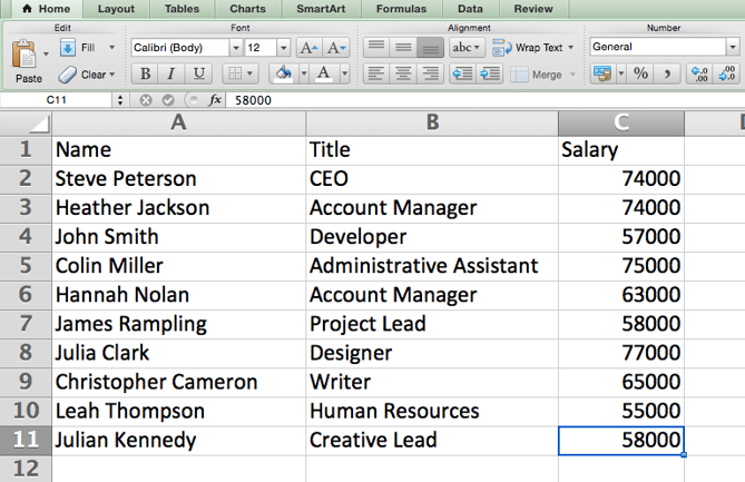
This will return the amount of the worths within a desired variety of cells that all meet one standard. For example, =SUMIF(C 3: C 12,"> 70,000") would return the amount of worths between cells C 3 as well as C 12 from only the cells that are better than 70,000. Let's claim you want to establish the earnings you generated from a checklist of leads who are related to particular location codes, or determine the amount of certain staff members' salaries-- yet only if they drop above a certain amount.

With the SUMIF feature, it does not have to be-- you can easily build up the sum of cells that fulfill certain criteria, like in the income example over. The formula: =SUMIF(range, requirements, [sum_range] Range: The variety that is being tested utilizing your criteria. Requirements: The criteria that figure out which cells in Criteria_range 1 will be totaled [Sum_range]: An optional variety of cells you're mosting likely to accumulate in addition to the initial Variety got in.

In the example listed below, we wanted to compute the sum of the wages that were more than $70,000. The SUMIF feature built up the dollar amounts that exceeded that number in the cells C 3 with C 12, with the formula =SUMIF(C 3: C 12,"> 70,000"). The TRIM formula in Excel is represented =TRIM(text).

What Does Excel Formulas Do?

For example, if A 2 consists of the name" Steve Peterson" with undesirable rooms prior to the given name, =TRIM(A 2) would certainly return "Steve Peterson" without rooms in a brand-new cell. Email and file sharing are fantastic tools in today's workplace. That is, up until one of your coworkers sends you a worksheet with some actually cool spacing.

Instead than meticulously getting rid of and also adding spaces as required, you can cleanse up any type of uneven spacing utilizing the TRIM function, which is used to remove extra spaces from information (with the exception of solitary rooms in between words). The formula: =TRIM(message). Text: The message or cell from which you want to remove spaces.

To do so, we entered =TRIM("A 2") right into the Solution Bar, as well as duplicated this for each name below it in a new column alongside the column with undesirable areas. Below are a few other Excel formulas you might find valuable as your data management requires expand. Let's say you have a line of text within a cell that you intend to damage down right into a few different segments.

Objective: Made use of to draw out the initial X numbers or personalities in a cell. The formula: =LEFT(message, number_of_characters) Text: The string that you want to extract from. Number_of_characters: The number of personalities that you desire to draw out starting from the left-most character. In the instance listed below, we went into =LEFT(A 2,4) into cell B 2, and replicated it right into B 3: B 6.

Objective: Made use of to draw out personalities or numbers in the center based upon placement. The formula: =MID(message, start_position, number_of_characters) Text: The string that you desire to draw out from. Start_position: The setting in the string that you wish to begin drawing out from. As an example, the very first setting in the string is 1.

9 Simple Techniques For Countif Excel

In this instance, we got in =MID(A 2,5,2) into cell B 2, as well as replicated it into B 3: B 6. That enabled us to remove the two numbers starting in the 5th placement of the code. Purpose: Utilized to remove the last X numbers or characters in a cell. The formula: =RIGHT(text, number_of_characters) Text: The string that you want to remove from.

excel formulas disappeared formulas excel portugues para ingles excel formulas keep disappearing